How it differs from ordinary image annotation
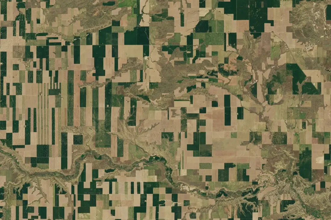
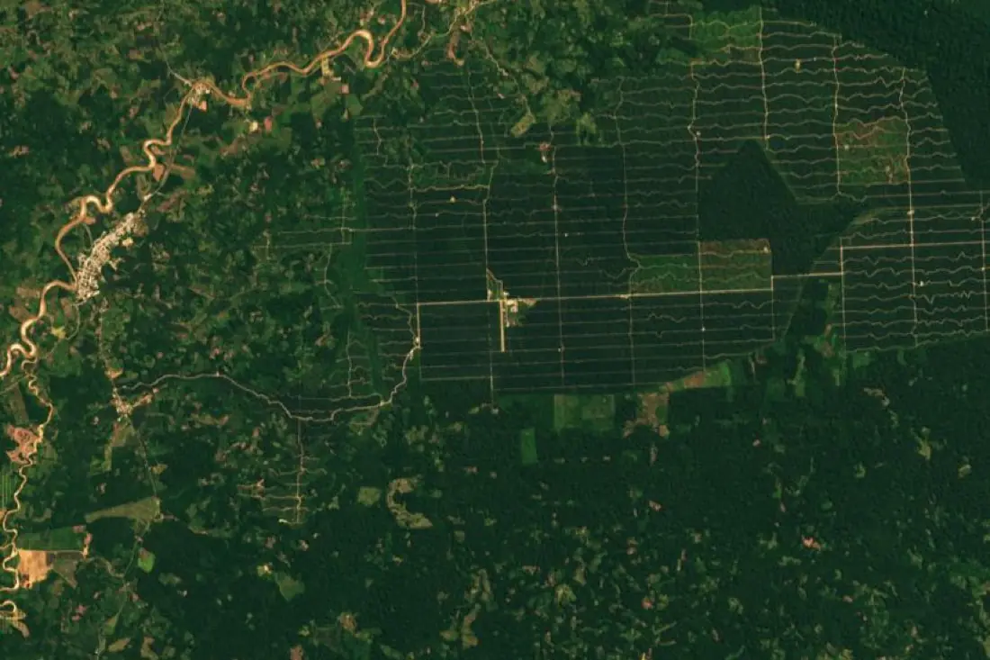
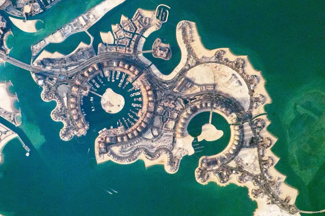
Annotating a satellite scene looks like annotating any photo: draw a shape, pick a class. Five things make it a different job.
- Every label has a place on Earth. Labels are stored in map coordinates, in a coordinate reference system (CRS) such as WGS 84 or a UTM zone, not only as pixel positions. That is what lets them line up with other data and with the next image of the same place.
- Scenes are huge. One Sentinel-2 tile covers 110 × 110 km. Scenes are cut into tiles for labeling, and the labels are stitched back without seams or duplicates at tile edges.
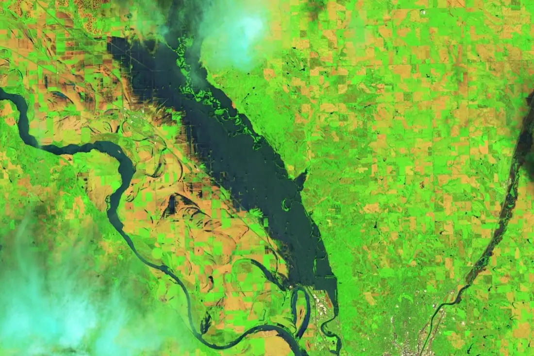
- There is more than red, green and blue. Multispectral sensors add near-infrared and shortwave-infrared bands. Annotators switch between band combinations to see vegetation, water and burn scars that a true-colour view hides.
- Resolution sets the limit. At 10 m a pixel is larger than a car. A class list has to match what the imagery can actually show, or annotators end up guessing.
- Time matters. Crop type, harvest and change tasks need several dates of the same place, labeled the same way every time.
Clouds, cloud shadow, haze and off-nadir lean (tall buildings leaning away from their footprint) add their own rules. A good guideline says how each one is handled before labeling starts.
Imagery types and what each can show
The imagery decides which classes are possible. Most projects use one of four kinds, sometimes together.
| Imagery | Typical resolution | Good for |
|---|---|---|
| Very-high-resolution optical (commercial satellite, aerial) | 0.3–1 m | Buildings, roads, vehicles, damage, small fields |
| Multispectral (Sentinel-2, Landsat 8/9) | 10–30 m | Crop type, land cover, water, burn scars, forest loss |
| Radar, SAR (Sentinel-1, commercial) | 1–20 m | Floods, change and ships, through cloud and at night |
| Elevation and LiDAR | Point clouds, DSM, DTM | Canopy height, structures, 3D objects |
Sentinel-1, Sentinel-2 and Landsat are free under open licences, which makes them the default for large areas and long time series. Commercial very-high-resolution imagery is bought per square kilometre and is needed when the objects are small.
Types of satellite annotation
The label geometry follows from what the model has to output.
- Polygons outline each object separately (one field, one building). Used for instance segmentation and for vector map layers.
- Segmentation masks give every pixel a class (water, forest, built-up). Used for semantic segmentation and land cover.
- Bounding boxes, axis-aligned or rotated (oriented), mark objects for detection models. Rotated boxes fit ships, vehicles and buildings that are not aligned with the image grid.
- Points mark objects that only need counting or locating: trees, wells, vehicles.
- Lines follow roads, rivers, field edges and power lines.
- Scene and time-series labels classify a whole tile, or give the date an event happened (a harvest, a clear-cut, a flood peak).
Formats and coordinate systems
Agree the delivery format and the CRS before the first label is drawn. Converting afterwards is where alignment errors creep in.
- Vector: GeoJSON, GeoPackage or Shapefile, with class and attributes per feature.
- Raster: Cloud-Optimized GeoTIFF masks on exactly the same pixel grid as the source image.
- Computer vision: COCO, YOLO or Pascal VOC, in pixel coordinates per tile, with the tile’s georeference kept so labels can be mapped back to the ground.
The labeling guideline
The guideline is the most important document in an annotation project. Two annotators reading it should draw the same thing. It should cover:
- A definition of every class, with example images of clear cases and of the edge cases.
- The minimum mapping unit: the smallest object that gets its own label.
- How to treat cloud, shadow and missing data. A dedicated class is better than a guess.
- What to do when the imagery cannot settle a case: flag it, never invent it.
- Which date or band combination is the reference when dates disagree.
Quality control
Labels are checked against a reviewed sample before delivery. The useful numbers are per class: precision and recall, or intersection over union (IoU) for shapes. Overall accuracy hides problems. A dataset can be 95% correct overall and still get a rare class, often the one that matters, wrong half the time.
For larger projects, a share of the area is labeled twice by different annotators. Where they disagree, the guideline is usually unclear, and fixing it there is cheaper than fixing labels later.
What drives the cost
- Area and density: a square kilometre of city holds far more objects than a square kilometre of forest.
- Classes: how many, and how hard they are to tell apart.
- Dates: every extra date multiplies the work, although later dates go faster once the first is done.
- Geometry: points are faster than boxes, boxes faster than polygons, polygons faster than pixel-accurate masks.
- Imagery: free Sentinel and Landsat data, or commercial imagery bought per square kilometre.
- Review depth: the size of the checked sample and whether areas are labeled twice.
Common mistakes
- Asking for classes the resolution cannot show, such as single trees in 10 m imagery.
- Mixing seasons or dates without saying so, so the same field gets two different labels.
- No “unknown” or “cloud” class, which forces annotators to guess.
- Training and test areas next to each other. Neighbouring tiles look alike, so test scores come out too high. Split by region instead.
- Reprojecting labels without checking they still line up with the imagery.
Written by IKT Spīdolas. See also: Drone image annotation: a practical guide.